You are here: CLASSE Wiki>CHESS/Maia Web>GeoPIXE>IntroGeoPIXEWorkflowOverview (21 Aug 2018, ArthurWoll)Edit Attach
Intro: GeoPIXE: Workflow overview
The resources on this page are intended to introduce the general process of working up XRF data in GeoPIXE. The topics referenced on this page are explained in greater detail in their own videos (links referenced in the video are also found on the main GeoPIXE tutorials page).Video
General outline of workflow steps
1. Collect calibration foil data (raw blog files) 2. Collect sample data (raw blog files) 3. Calculate flux/charge calibration from foil data (needs to be done for each foil- when energy is changed, etc.) 4. Import raw blog files as spectra and apply flux/charge & energy calibrations 5. Fit the spectra (adjust yields calculation; adjust elements, background, cuts, etc.) 6. Generate a new DA matrix 7. Generate a processed set of XRF elemental maps from the raw data using the new DA matrix in the Sort EVT window 8. Examine the maps in the main GeoPIXE window and locate regions where fit needs refinement 9. If fit is adjusted, regenerate a DA matrix and re-process the raw data to give new elemental maps 10. Save the elemental maps (qualitative and/or quantitative)Notes
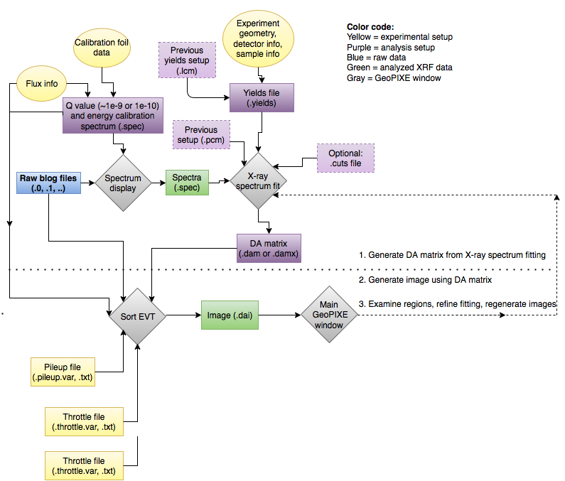
Here is a schematic diagram showing how all the different data analysis processes and windows in GeoPIXE contribute to generating a processed set of XRF elemental maps.
- Yellow ovals represent information about your experiment that are set while the data is being collected, but are not digital GeoPIXE files (e.g., sample geometry, how flux was measured, which calibration foils were used, etc.)
- Rectangles represent types of digital files
- Yellow rectangles represent information about your experiment that are set while the data is being collected that are saved as digital GeoPIXE files (pileup and throttle files)
- Fields in blue represent raw data
- Fields in green represent analyzed XRF data
- Fields in purple represent files related to data analysis
- Gray diamonds are GeoPIXE windows
Previous: IntroGeoPIXELaunchingGeoPIXE
Next: IntroGeoPIXEFileSelectGeneral
-- LouisaSmieska - 05 May 2016
Edit | Attach | Print version | History: r5 < r4 < r3 < r2 | Backlinks | View wiki text | Edit wiki text | More topic actions
Topic revision: r5 - 21 Aug 2018, ArthurWoll
- Webs
-
 ACC
ACC
-
 ACL
ACL
-
 Bunch
Bunch
-
 CBB
CBB
-
 NSF
NSF
-
 CBETA
CBETA
-
 CESR
CESR
-
 Private
-
 CHESS
CHESS
-
 FMB
FMB
-
 Maia
Maia
-
 XIMG
XIMG
-
 XLEAP
XLEAP
-
 CHEXS
CHEXS
-
 CLASSE
-
 Inventory
-
 CLEO
CLEO
-
 CMSPhase2MREFC
-
 Computing
-
 Blogs
Blogs
-
 Newsletter
-
 Cosmology
-
 DarkPhoton
-
 ERL
ERL
-
 EngineeringDesignDrafting
-
 G2
G2
-
 HEP
HEP
-
 DBSWorkshop
-
 SWIG
SWIG
-
 HLLHCCMSMREFC
-
 HMF
HMF
-
 HumanResources
-
 Private
-
 ILC
ILC
-
 Americas
-
 CesrTA
-
 Proposal
-
 DampingRings
-
 AreaLeaders
-
 CTA09
CTA09
-
 ILCDR06
-
 ILCDR07_KEK
-
 ILCDR08
-
 S3TaskForce
-
 WWS
WWS
-
 MacCHESS
-
 Main
Main
-
 People
-
 PhotocathodeBrightBeams
-
 REU
REU
-
 SRF
SRF
-
 Safety
-
 Sandbox
-
 TestWeb
-
 System
-
 Theory
-
 Communications
-
 Documents
-
 Phase2MREFC
-
 WebDev
-
 XLEAP
XLEAP
 Copyright © by the contributing authors. All material on this collaboration platform is the property of the contributing authors.
 Ideas, requests, problems regarding CLASSE Wiki? Send feedback
